Should You Shoot Free Throws Underhand?
This week’s FiveThirtyEight.com Riddler:
Consider the following simplified model of free throws. Imagine the rim to be a circle (which we’ll call C) that has a radius of 1, and is centered at the origin (the point (0,0)). Let V be a random point in the plane, with coordinates X and Y, and where X and Y are independent normal random variables, with means equal to zero and each having equal variance — think of this as the point where your free throw winds up, in the rim’s plane. If V is in the circle, your shot goes in. Finally, suppose that the variance is chosen such that the probability that V is in C is exactly 75 percent (roughly the NBA free-throw average).
But suppose you switch it up, and go granny-style, which in this universe eliminates any possible left-right error in your free throws. What’s the probability you make your shot now? (Put another way, calculate the probability that Y is less than 1 in absolute value.)
Understanding the Problem
The (X, Y) coordinate of a regular overhand shot is determined by two random draws from independent and identically distributed normal distributions. We are given the mean but need to calculate the variance such that the probability of making a shot is 75 percent (the NBA average).
Put differently, we need to find the variance of the normal distributions such that the distance between the shot’s (X,Y) location and the origin is less than one. We can express the square of this distance as:
\[ D^2 = X^2 + Y^2 \]
The distance is the sum of the square of two random normal variables (we should be taking the square root to find distance, but since we really care about whether the distance is less than 1 in absolute value, we can get away with focusing on the square). We can model distance squared as a random variable with a gamma distribution that has a shape parameter equal to 1 and a scale parameter equal to \(2 \sigma^2\), where \(\sigma\) is the standard deviation of the X and Y normal distributions.
Our job is to find the value of \(\sigma\) such that the cumulative probability of distance being less than one is 75 percent. Once we find the calibrated standard deviation, we can go back to our normal distribution of Y and find the cumulative probability that Y is less than one in absolute value.
Calibrating the Probability Distribution
We need to calibrate the gamma distribution such that the cumulative probability of a shot with distance less than one is 75 percent. This is simpler to visualize if we think about what the cumulative distribution function of the calibrated gamma distribution should look like:
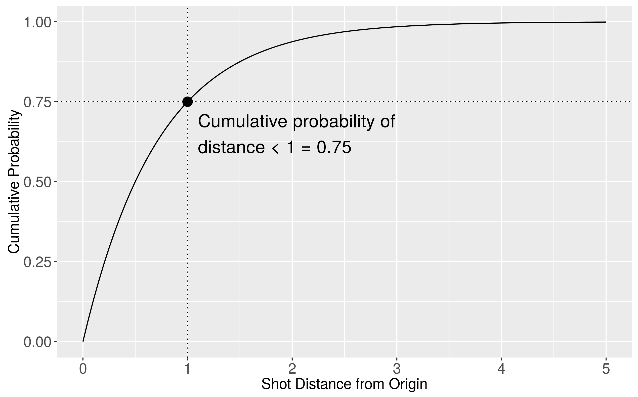
There are closed-form solutions that you can write down to solve the CDF of the gamma distribution, but as a cheap substitute we can calibrate it programmatically. Remember, we are looking for the right \(\sigma\) value that gives us the proper CDF.
- Define a range of \(\sigma\) values over which we will search.
- For each candidate \(\sigma\) value, calculate the CDF at 1.
- Choose the value of \(\sigma\) that produces a CDF(1) as close to 0.75 as possible.
There are efficient search algorithms you can use for this, but since this is a small-scale problem, I started with a large range and a coarse search grid, found an approximate right answer, and then ran the search again over a small range with a fine search grid. I find that the proper value of \(\sigma\) is 0.6005612.
Verify by Simulation
As a check of our intuition, we can use this calibrated value of \(\sigma\) to simulate a series of free throw shots and see how many we “make.” To do so, we take N draws from the X and Y i.i.d. normal distributions, calculate the distance of each pair of draws, and see how many have distance less than one.
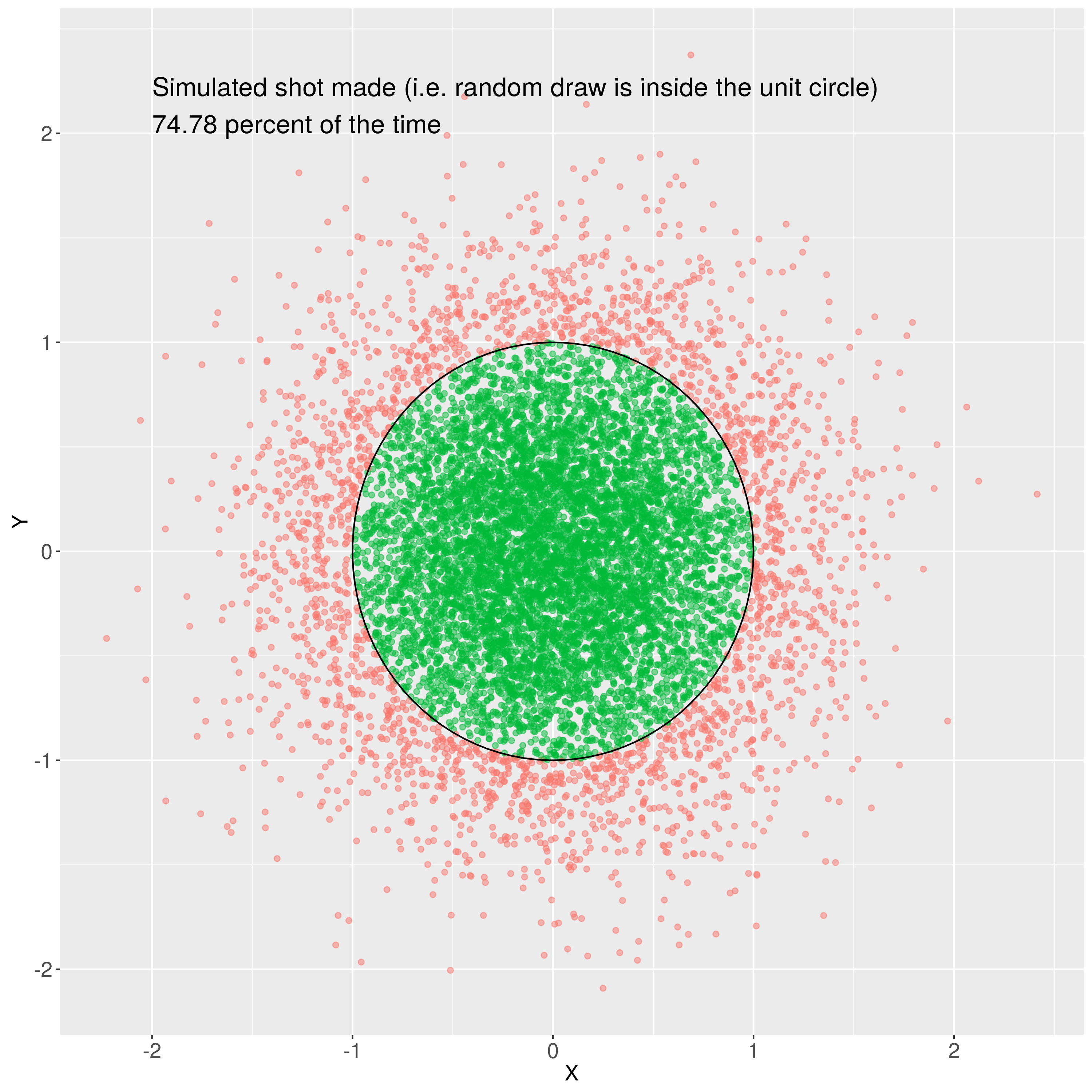
This looks good! For N = 10,000, we “make” a shot about 74.8 percent of the time. We would expect some noise as even for large N there is still some randomness in the shot draws, but this tells us that our \(\sigma\) value is calibrated correctly.
Solution: Should You Shoot Underhand?
Now we’re close to the payoff. We’ve calibrated the variance of our X and Y distributions and need to find the probability than Y is less than one in absolute value. We can see this easily from the cumulative probability density function of our Y distribution:
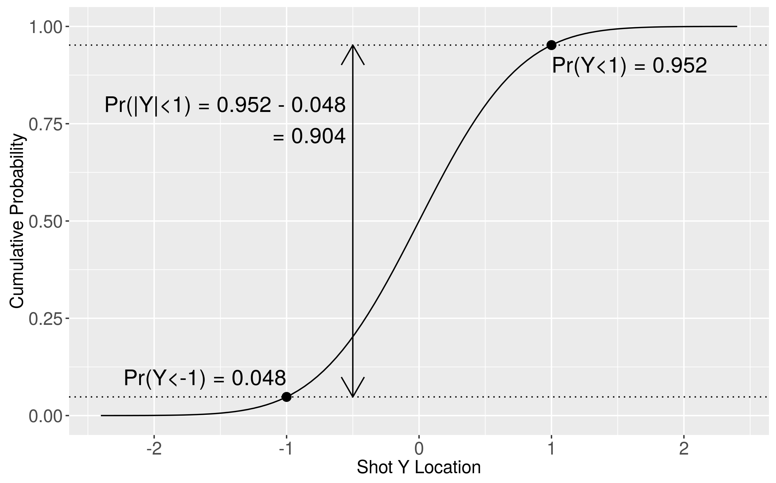
The probability that Y is less than 1 in absolute value is equal to: \[ Pr( \vert Y \vert <1) = Pr(Y<1) - Pr(Y<-1) = 0.9520545 - 0.04794548 = 0.9041090 \] That is, if you shoot your free throws underhand, you should expect to make your shot 90.41090 percent of the time.
Extension: No Free Lunches
In basketball as in life, there are no free lunches. Suppose shooting underhanded really did eliminate the variance from your shot’s X location, but at the cost of increasing the variance of your shot’s Y location. How much would the variance of Y have to increase before you would be indifferent between shooting normally and shooting underhanded?
Let’s call the new, high variance Y location Y’. The key here is to select a variance of Y’ such that the cumulative probability between -1 and 1 is 0.75. We can use the same search algorithm as we did when calibrating our gamma distribution. Here, I find that the variance of Y’ is 0.8693011. The cumulative distribution function of Y’ helps visualize the change (the original CDF is plotted in light gray):
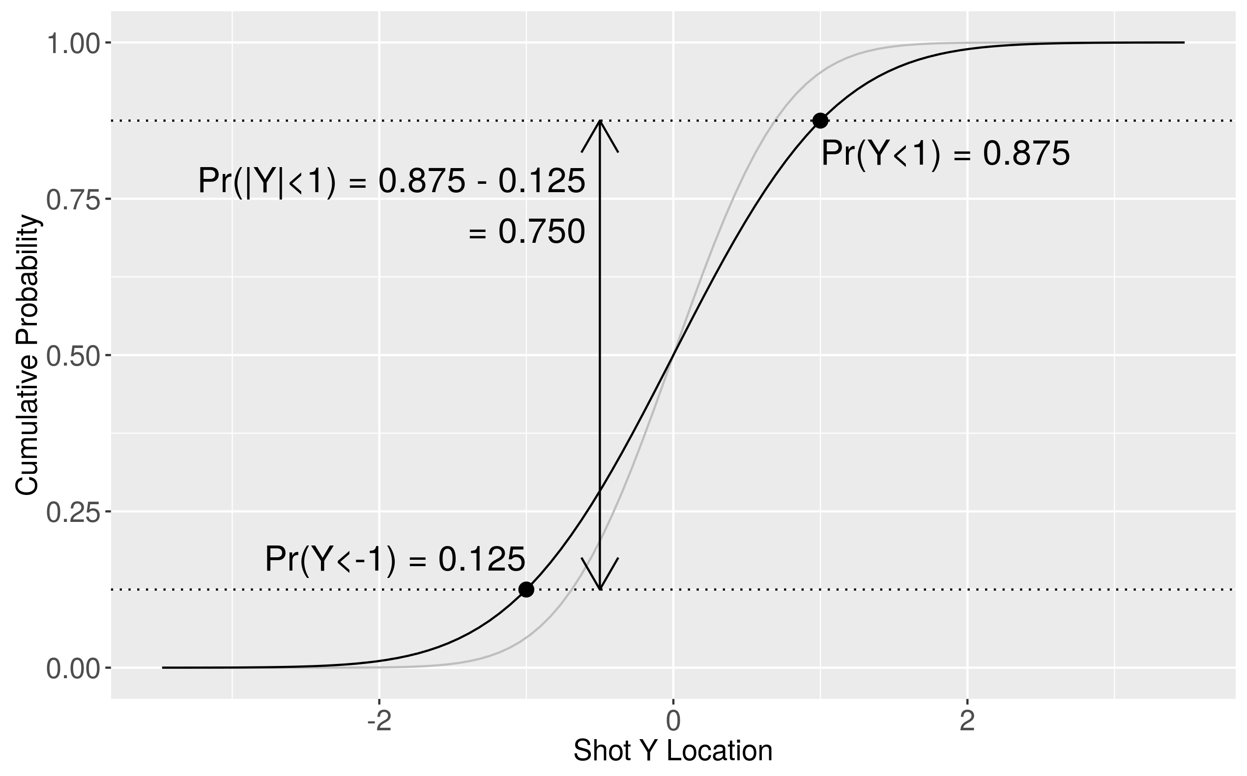
In other words, the variance of a shot’s Y location would have to increase by 44.74813 percent: \[ \frac{\text{var}(Y’)}{\text{var}(Y)}-1 = \frac{0.8693011}{0.6005612} - 1 = 44.74813 \% \]
Discussion